Fine-tuning a pre-trained model

Warning

Finetuning is currently only available for the PET architecture.

This is a simple example for fine-tuning PET-MAD (or a general PET model), that can be used as a template for general fine-tuning with metatrain. Fine-tuning a pretrained model allows you to obtain a model better suited for your specific system. You need to provide a dataset of structures that have been evaluated at a higher reference level of theory, usually DFT. Fine-tuning a universal model such as PET-MAD allows for reasonable model performance even if little training data is available. It requires using a pre-trained model checkpoint with the mtt train command and setting the new targets corresponding to the new level of theory in the options.yaml file.

In order to obtain a pretrained model, you can use a PET-MAD checkpoint from huggingface

wget https://huggingface.co/lab-cosmo/pet-mad/resolve/v1.1.0/models/pet-mad-v1.1.0.ckpt

Next, we set up the options.yaml file. Here we specify to fine-tune on a small model dataset containing structures of ethanol, labelled with energies and forces. We can specify the fine-tuning method in the finetune block in the training options of the architecture. Here, the basic full option is chosen, which finetunes all weights of the model. All available fine-tuning methods are found in the concepts page Fine-tuning. This section discusses implementation details, options and recommended use cases. Other fine-tuning options can be simply substituted in this script, by changing the finetune block.

Note

Since our dataset has energies and forces obtained from reference calculations, different from the reference of the pretrained model, it is recommended to create a new energy head. Using this so-called energy variant can be simply invoked by requesting a new target in the options file. Follow the nomenclature energy/{yourname}.

Furthermore, you need to specify the checkpoint, that you want to fine-tune in the read_from option.

A simple options-ft.yaml file for this task could look like this:

architecture:
  name: pet
  training:
    batch_size: 8
    num_epochs: 10
    learning_rate: 1e-3
    warmup_fraction: 0.01
    finetune:
      method: full
      read_from: pet-mad-v1.1.0.ckpt
      inherit_heads:
        energy/finetune: energy # inherit weights from the "energy" head

training_set:
  systems:
    read_from: ethanol_reduced_100.xyz
    reader: ase
    length_unit: angstrom
  targets:
    energy/finetune:
      quantity: energy
      read_from: ethanol_reduced_100.xyz
      reader: ase
      key: energy
      unit: eV
      description: "pbe energy ethanol"
      forces:
        read_from: ethanol_reduced_100.xyz
        reader: ase
        key: forces

validation_set: 0.1
test_set: 0.1

In this example, we specified a low number of num_epochs and a relatively high learning_rate, for short compilation time. Usually, the learning_rate is chosen to be relatively low. Typically lower, than the learning_rate that the model has been per-trained on. to stabilise training.

Warning

Note that in targets we use the energy/finetune head, differing from the default energy head. This means, that the model creates a new head with a new composition model for the new reference energies provided in your dataset. While the old energy reference is still available, it is rendered useless, as we trained all weights of the model. If you want to obtain a model with multiple energy heads, you can simply train on multiple energy references simultaneously. This and other more advanced fine-tuning strategies are discussed in Fine-tuning concepts.

We assumed that the pre-trained model is trained on the dataset ethanol_reduced_100.xyz in which energies are written in the energy key of the info dictionary of the dataset. Additionally, forces should be provided with corresponding keys which you can specify in the options-ft.yaml file under targets. Further information on specifying targets can be found in the data section of the Training YAML Reference.

Note

It is important that the length_unit is set to angstrom and the energy unit is eV in order to match the units of your reference data.

After setting up your options-ft.yaml file, you can then simply run:

mtt train options-ft.yaml -o model-ft.pt

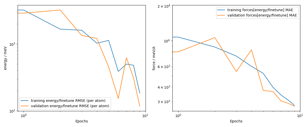
You can check finetuning training curves by parsing the train.csv that is written by mtt train. We remove the old outputs folder from other examples, which is not necessary for the normal usage.

import glob
import subprocess

import ase.io
import matplotlib.pyplot as plt
import numpy as np
from metatomic.torch.ase_calculator import MetatomicCalculator

# Here, we get the PET-MAD ckpt, run ``mtt train`` as a subprocess, and delete the old
# outputs folder.
subprocess.run(
    [
        "wget",
        "https://huggingface.co/lab-cosmo/pet-mad/resolve/v1.1.0/models/pet-mad-v1.1.0.ckpt",
    ]
)
subprocess.run(["rm", "-rf", "outputs"])
subprocess.run(["mtt", "train", "options-ft.yaml", "-o", "model-ft.pt"], check=True)

CompletedProcess(args=['mtt', 'train', 'options-ft.yaml', '-o', 'model-ft.pt'], returncode=0)

csv_path = glob.glob("outputs/*/*/train.csv")[-1]
with open(csv_path, "r") as f:
    header = f.readline().strip().split(",")
    f.readline()  # skip units row

# Build dtype
dtype = [(h, float) for h in header]

# Load data as plain float array
data = np.loadtxt(csv_path, delimiter=",", skiprows=2)

# Convert to structured
structured = np.zeros(data.shape[0], dtype=dtype)
for i, h in enumerate(header):
    structured[h] = data[:, i]

Now, let’s plot the learning curves.

training_energy_RMSE = structured["training energy/finetune RMSE (per atom)"]
training_forces_MAE = structured["training forces[energy/finetune] MAE"]
validation_energy_RMSE = structured["validation energy/finetune RMSE (per atom)"]
validation_forces_MAE = structured["validation forces[energy/finetune] MAE"]

fig, axs = plt.subplots(1, 2, figsize=(12, 5))

axs[0].plot(training_energy_RMSE, label="training energy/finetune RMSE (per atom)")
axs[0].plot(validation_energy_RMSE, label="validation energy/finetune RMSE (per atom)")
axs[0].set_xlabel("Epochs")
axs[0].set_ylabel("energy / meV")
axs[0].set_xscale("log")
axs[0].set_yscale("log")
axs[0].legend()
axs[1].plot(training_forces_MAE, label="training forces[energy/finetune] MAE")
axs[1].plot(validation_forces_MAE, label="validation forces[energy/finetune] MAE")
axs[1].set_ylabel("force / meV/A")
axs[1].set_xlabel("Epochs")
axs[1].set_xscale("log")
axs[1].set_yscale("log")
axs[1].legend()
plt.tight_layout()
plt.show()

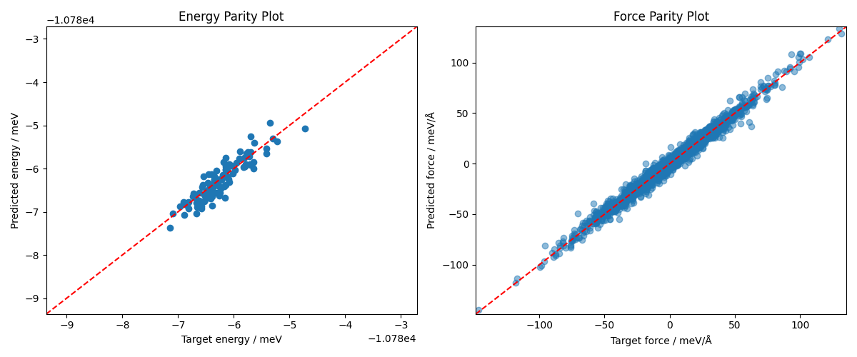
You can see that the validation loss still decreases, however, for the sake of brevity of this exercise we only finetuned for a few epochs. As further check for how well your fine-tuned model performs on a dataset of choice, we can check the parity plots for energy and force (see Model validation with parity plots). For evaluation, we can compare performance of our fine-tuned model and the base model PET-MAD. Using mtt eval we can simply evaluate our new energy head, by specifying it in the options-ft-eval.yaml:

systems: ethanol_reduced_100.xyz
targets:
  energy/finetune:
    key: energy
    unit: eV
    forces:
      key: forces

and then run

mtt eval model-ft.pt options-ft-eval.yaml -o output-ft.xyz

Then you can simply read the predicted energies in the headers of the xyz file. Another possibility is to load your fine-tuned model model-ft.pt as metatomic model and evaluate energies and forces with ASE in Python.

targets = ase.io.read(
    "ethanol_reduced_100.xyz",
    format="extxyz",
    index=":",
)
calc_ft = MetatomicCalculator(
    "model-ft.pt", variants={"energy": "finetune"}, extensions_directory=None
)  # specify variant suffix here

e_targets = np.array(
    [frame.get_total_energy() / len(frame) for frame in targets]
)  # target energies
f_targets = np.array(
    [frame.get_forces().flatten() for frame in targets]
).flatten()  # target forces

for frame in targets:
    frame.set_calculator(calc_ft)

e_predictions = np.array(
    [frame.get_total_energy() / len(frame) for frame in targets]
)  # predicted energies
f_predictions = np.array(
    [frame.get_forces().flatten() for frame in targets]
).flatten()  # predicted forces

/home/docs/checkouts/readthedocs.org/user_builds/metatrain/checkouts/943/examples/0-beginner/02-fine-tuning.py:256: FutureWarning: Please use atoms.calc = calc
  frame.set_calculator(calc_ft)
/home/docs/checkouts/readthedocs.org/user_builds/metatrain/envs/943/lib/python3.13/site-packages/metatomic/torch/ase_calculator.py:903: RuntimeWarning: invalid value encountered in scalar add
  (stress[1, 2] + stress[2, 1]) / 2.0,
/home/docs/checkouts/readthedocs.org/user_builds/metatrain/envs/943/lib/python3.13/site-packages/metatomic/torch/ase_calculator.py:904: RuntimeWarning: invalid value encountered in scalar add
  (stress[0, 2] + stress[2, 0]) / 2.0,

fig, axs = plt.subplots(1, 2, figsize=(12, 5))

# Parity plot for energies
axs[0].scatter(e_targets, e_predictions, label="FT")
axs[0].axline((np.min(e_targets), np.min(e_targets)), slope=1, ls="--", color="red")
axs[0].set_xlabel("Target energy / meV")
axs[0].set_ylabel("Predicted energy / meV")
min_e = np.min(np.array([e_targets, e_predictions])) - 2
max_e = np.max(np.array([e_targets, e_predictions])) + 2
axs[0].set_title("Energy Parity Plot")
axs[0].set_xlim(min_e, max_e)
axs[0].set_ylim(min_e, max_e)

# Parity plot for forces
axs[1].scatter(f_targets, f_predictions, alpha=0.5, label="FT")
axs[1].axline((np.min(f_targets), np.min(f_targets)), slope=1, ls="--", color="red")
axs[1].set_xlabel("Target force / meV/Å")
axs[1].set_ylabel("Predicted force / meV/Å")
min_f = np.min(np.array([f_targets, f_predictions])) - 2
max_f = np.max(np.array([f_targets, f_predictions])) + 2
axs[1].set_title("Force Parity Plot")
axs[1].set_xlim(min_f, max_f)
axs[1].set_ylim(min_f, max_f)
fig.tight_layout()
plt.show()

Further fine-tuning examples can be found in the AtomisticCookbook